46. Job Search V: Risk-Sensitive Preferences#
GPU
This lecture was built using a machine with access to a GPU.
Google Colab has a free tier with GPUs that you can access as follows:
Click on the “play” icon top right
Select Colab
Set the runtime environment to include a GPU
46.1. Overview#
Risk-sensitive preferences are a common addition to various types of dynamic programming problems.
This lecture gives an introduction to risk-sensitive recursive preferences via job search.
Some motivation is given below.
46.2. Outline#
In real-world job-related decisions, individuals and households care about risk.
For example, some individuals might prefer to take a moderate offer already in hand over the risky possibility of a higher offer in the next period, even without discounting future payoffs.
(A bird in the hand is worth two in the bush, etc.)
In previous job search lectures in this series, we inserted some degree of risk aversion by adding a concave flow utility function \(u\).
Unfortunately, this strategy does not isolate preferences over the kind of risk we described above.
This is because adding a concave utility function changes the agent’s preferences in other ways, such as in their desire for consumption smoothing.
Hence, if we want to study the pure effects of risk, we need a different solution.
One possibility is to add risk-sensitive preferences.
Here we show how this can be done and study what effects it has on agent choices.
We’ll use JAX and the QuantEcon library:
!pip install quantecon jax
We use the following imports.
import jax
import jax.numpy as jnp
from jax import lax
import quantecon as qe
from typing import NamedTuple
import numpy as np
import matplotlib.pyplot as plt
Matplotlib is building the font cache; this may take a moment.
46.3. Introduction to risk-sensitivity#
Let’s start our discussion in a static environment.
If \(Y\) is a random payoff and an agent’s evaluation of the payoff is \(e := \mathbb{E} Y\), then we say that the agent is risk neutral.
Sometimes we want to model agents as risk averse.
One way to do this is to change their evaluation of the payoff \(Y\) to
where \(\theta\) is a number satisfying \(\theta < 0\).
The value \(e_{\theta}\) is sometimes called the entropic risk-adjusted expectation of \(Y\).
46.3.1. A Gaussian example#
One way to see the impact is to suppose that \(Y\) has the normal distribution \(N(\mu, \sigma^2)\), so that its mean is \(\mu\) and its variance is \(\sigma^2\).
For this \(Y\) we aim to compute the risk-adjusted expectation.
This becomes straightforward if we recognize that \(\mathbb{E}[\exp(\theta Y)]\) is the moment generating function (MGF) of the normal distribution.
Using the well-known expression for the MGF of the normal distribution, we get
Therefore,
Simplifying yields
We see immediately that the agent prefers a higher average payoff \(\mu\).
At the same time, given that \(\theta < 0\), the risk-adjusted expectation decreases in \(\sigma\).
In particular, \(e_\theta\) decreases as risk increases.
Here is a visualization of \(e_\theta\) as a function of \(\mu\) and \(\sigma\) using a contour plot, with \(\theta=-1\).
theta = -1

mu_vals = np.linspace(-2, 5, 200)
sigma_vals = np.linspace(0.1, 3, 200)
mu_grid, sigma_grid = np.meshgrid(mu_vals, sigma_vals)

e_theta = mu_grid + (theta * sigma_grid**2) / 2

# Create contour plot
fig, ax = plt.subplots(figsize=(10, 8))
contour = ax.contour(
    mu_grid, sigma_grid, e_theta, levels=20, colors='black', linewidths=0.5
)
contourf = ax.contourf(
    mu_grid, sigma_grid, e_theta, levels=20, cmap='viridis'
)
ax.clabel(contour, inline=True, fontsize=8)
cbar = plt.colorbar(contourf, ax=ax)
cbar.set_label(r'$e_\theta$', rotation=0, fontsize=12)

ax.set_xlabel(r'$\mu$ (mean)', fontsize=12)
ax.set_ylabel(r'$\sigma$ (standard deviation)', fontsize=12)
plt.tight_layout()
plt.show()
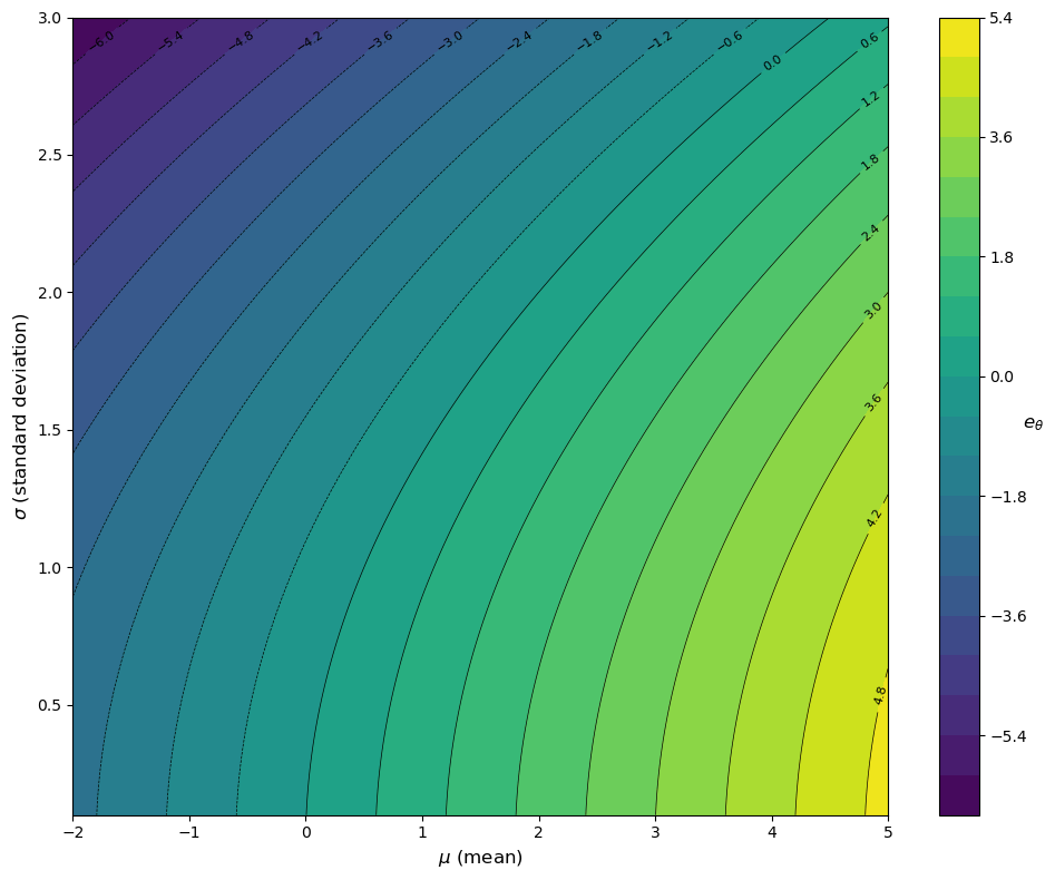
Again, we see that the agent prefers a higher average payoff but dislikes risk.
46.3.2. A more general case#
The preceding analysis relies on the Gaussian (normal) assumption to get an analytical solution.
We can investigate all other cases using simulation.
For example, suppose that \(Y\) has the Beta\((a, b)\) distribution.
Here we set \(a=b=2.0\) and calculate \(e_{\theta}\) using Monte Carlo
The method is:
sample \(Y_1, \ldots, Y_n\) from Beta\((2,2)\)
replace \(\mathbb{E}\) with an average over \(\exp(\theta Y_i)\)
We do this for \(\theta\) in a grid of 100 points between \(-2\) and \(-0.1\).
Here is a plot of \(e_{\theta}\) against \(\theta\).
import jax
import jax.numpy as jnp
import matplotlib.pyplot as plt

# Set parameters
a, b = 2.0, 2.0
mc_size = 1_000_000  # Large number of Monte Carlo samples
theta_grid = jnp.linspace(-2, -0.1, 100)

# Draw samples from Beta(2, 2) distribution using JAX
key = jax.random.PRNGKey(1234)
Y_samples = jax.random.beta(key, a, b, shape=(mc_size,))

# Define function to compute e_theta for a single theta value
def compute_e_theta(theta):
    """Compute e_theta = (1/theta) * ln(E[exp(theta * Y)])"""
    expectation = jnp.mean(jnp.exp(theta * Y_samples))
    return (1 / theta) * jnp.log(expectation)

# Vectorize over theta_grid using vmap
compute_e_theta_vec = jax.vmap(compute_e_theta)
e_theta_values = compute_e_theta_vec(theta_grid)

# Plot results
fig, ax = plt.subplots(figsize=(10, 6))
ax.plot(theta_grid, e_theta_values, linewidth=2)
ax.set_xlabel(r'$\theta$', fontsize=14)
ax.set_ylabel(r'$e_\theta$', fontsize=14)
ax.set_title(r'$e_\theta$ for $Y \sim \text{Beta}(2, 2)$', fontsize=14)
ax.axhline(y=0.5, color='black', linestyle='--',
           linewidth=1, label=r'$\mathbb{E}[Y] = 0.5$')
ax.legend(fontsize=12)
plt.tight_layout()
plt.show()
W1210 01:15:46.707857    2267 cuda_executor.cc:1802] GPU interconnect information not available: INTERNAL: NVML doesn't support extracting fabric info or NVLink is not used by the device.
W1210 01:15:46.711386    2197 cuda_executor.cc:1802] GPU interconnect information not available: INTERNAL: NVML doesn't support extracting fabric info or NVLink is not used by the device.
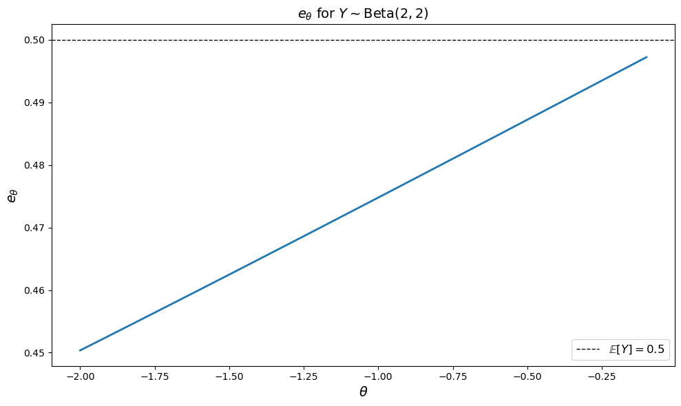
The plot shows how the risk-adjusted evaluation \(e_\theta\) changes with the risk aversion parameter \(\theta\).
As \(\theta \to 0\), the value \(e_\theta\) approaches the expected value of \(Y\), which is \(\mathbb{E}[Y] = \frac{a}{a+b} = \frac{2}{4} = 0.5\) for Beta(2,2).
This makes sense because when \(\theta \to 0\), the agent becomes risk neutral.
As \(\theta\) becomes more negative, \(e_\theta\) decreases.
This reflects that a more risk-averse agent values the uncertain payoff \(Y\) less than its expected value.
46.3.3. A mean preserving spread#
The next exercise asks you to study the impact of a mean-preserving spread on the risk-adjusted expectation.
Exercise 46.1
Keep \(Y \sim \text{Beta}(2, 2)\) and fix \(\theta = -2\).
Using Monte Carlo again, calculate
where \(X = Y + \sigma Z\) and \(Z\) is standard normal.
How does \(e_\theta\) change with \(\sigma\)?
Can you provide some intuition for what is happening (given that the agent is risk averse)?
Use a plot to illustrate your results.
Solution
Here’s our solution.
a, b = 2.0, 2.0
theta = -2.0
mc_size = 1_000_000  # Large number of Monte Carlo samples
sigma_grid = jnp.linspace(0.0, 1.0, 50)

# Set random seed for reproducibility
key = jax.random.PRNGKey(1234)
key_y, key_z = jax.random.split(key)

# Draw samples from Beta(2, 2) distribution
Y_samples = jax.random.beta(key_y, a, b, shape=(mc_size,))

# Draw standard normal samples (reused for all sigma values)
Z_samples = jax.random.normal(key_z, shape=(mc_size,))

# Define function to compute e_theta for a single sigma value
def compute_e_theta(sigma):
    """Compute e_theta for X = Y + sigma * Z"""
    # Compute X = Y + sigma * Z
    X_samples = Y_samples + sigma * Z_samples

    # Calculate E[exp(theta * X)] using Monte Carlo
    expectation = jnp.mean(jnp.exp(theta * X_samples))

    # Calculate e_theta
    return (1 / theta) * jnp.log(expectation)

# Vectorize over sigma_grid using vmap
compute_e_theta_vec = jax.vmap(compute_e_theta)
e_theta_values = compute_e_theta_vec(sigma_grid)

# Plot results
fig, ax = plt.subplots(figsize=(10, 6))
ax.plot(sigma_grid, e_theta_values, linewidth=2.5, label=r'$e_\theta(\sigma)$')
ax.set_xlabel(r'$\sigma$ (noise level)', fontsize=14)
ax.set_ylabel(r'$e_\theta$', fontsize=14)
ax.set_title(r'Risk-adjusted evaluation as noise increases', fontsize=14)
ax.axhline(y=e_theta_values[0], color='black', linestyle='--', linewidth=1,
           label=f'No noise: $e_\\theta$ = {e_theta_values[0]:.3f}')
ax.legend(fontsize=12)
plt.tight_layout()
plt.show()
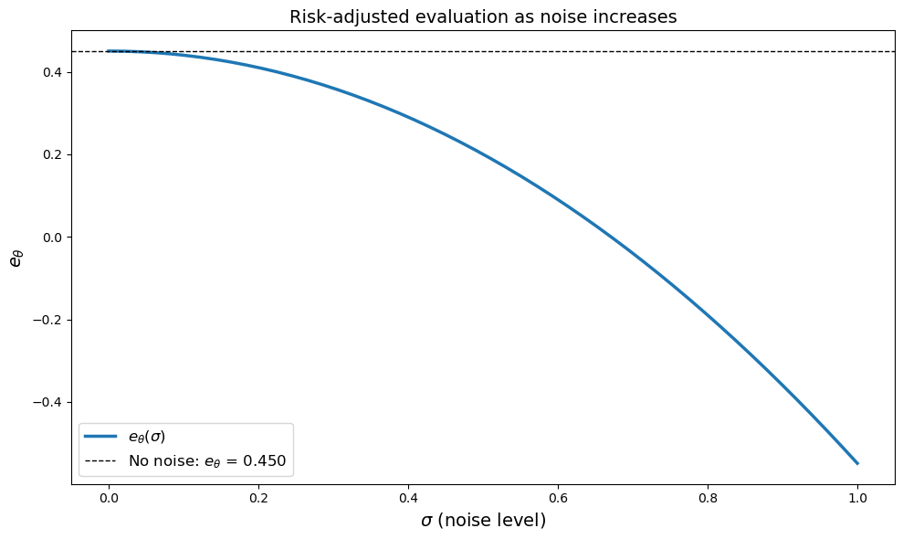
The plot clearly shows that \(e_\theta\) decreases monotonically as \(\sigma\) increases.
Since the agent is risk averse (\(\theta = -2 < 0\)), she dislikes uncertainty.
As we increase \(\sigma\), we get more volatility, since
At the same time, the expected value is unchanged, since
Hence the mean payoff doesn’t change with \(\sigma\).
In other words, the risk averse agent is not compensated for bearing additional risk.
This is why the valuation of the random payoff goes down.
46.4. Back to Job Search#
In the lecture Job Search IV: Fitted Value Function Iteration we studied a job search model with separation, Markov wage draws and fitted value function iteration.
The wage offer process is continuous and obeys
and \(\{Z_t\}\) is IID and standard normal.
Let’s now study the same model but replacing the assumption of risk neutral expectations with risk averse expectations.
In particular, the conditional expectation
from that lecture is replaced with
Otherwise the model is the same.
We now solve the dynamic program and study the impact of \(\theta\) on the reservation wage.
46.4.1. Setup#
Here’s a class to store parameters and default parameter values.
class Model(NamedTuple):
    c: float              # unemployment compensation
    α: float              # job separation rate
    β: float              # discount factor
    ρ: float              # wage persistence
    ν: float              # wage volatility
    θ: float              # risk aversion parameter
    w_grid: jnp.ndarray   # grid of points for fitted VFI
    z_draws: jnp.ndarray  # draws from the standard normal distribution

def create_mccall_model(
        c: float = 1.0,
        α: float = 0.1,
        β: float = 0.96,
        ρ: float = 0.9,
        ν: float = 0.2,
        θ: float = -1.5,
        grid_size: int = 100,
        mc_size: int = 1000,
        seed: int = 1234
    ):
    """Factory function to create a McCall model instance."""

    key = jax.random.PRNGKey(seed)
    z_draws = jax.random.normal(key, (mc_size,))

    # Discretize just to get a suitable wage grid for interpolation
    mc = qe.markov.tauchen(grid_size, ρ, ν)
    w_grid = jnp.exp(jnp.array(mc.state_values))

    return Model(c, α, β, ρ, ν, θ, w_grid, z_draws)
46.4.2. Bellman equations#
Our construction is a direct extension of the Bellman equations in Job Search IV: Fitted Value Function Iteration.
First we use the employed worker’s Bellman equation to express \(v_e(w)\) in terms of \((P_\theta v_u)(w)\):
We substitute into the unemployed agent’s Bellman equation to get:
We use value function iteration to solve for \(v_u\).
Then we compute the optimal policy: accept if \(v_e(w) ≥ u(c) + β(P_\theta v_u)(w)\)
Here’s the Bellman operator that updates \(v_u\).
def T(model, v):
    # Unpack model parameters
    c, α, β, ρ, ν, θ, w_grid, z_draws = model

    # Interpolate array represented value function
    vf = lambda x: jnp.interp(x, w_grid, v)

    def compute_expectation(w):
        # Use Monte Carlo to evaluate integral (P_θ v)(w)
        inner = jnp.mean(jnp.exp(θ * vf(w**ρ * jnp.exp(ν * z_draws))))
        return (1 / θ) * jnp.log(inner)

    compute_exp_all = jax.vmap(compute_expectation)
    P_θ_v = compute_exp_all(w_grid)

    d = 1 / (1 - β * (1 - α))
    accept = d * (w_grid + α * β * P_θ_v)
    reject = c + β * P_θ_v
    return jnp.maximum(accept, reject)
Here’s the solver:
@jax.jit
def vfi(
        model: Model,
        tolerance: float = 1e-6,   # Error tolerance
        max_iter: int = 100_000,   # Max iteration bound
    ):

    v_init = jnp.zeros(model.w_grid.shape)

    def cond(loop_state):
        v, error, i = loop_state
        return (error > tolerance) & (i <= max_iter)

    def update(loop_state):
        v, error, i = loop_state
        v_new = T(model, v)
        error = jnp.max(jnp.abs(v_new - v))
        new_loop_state = v_new, error, i + 1
        return new_loop_state

    initial_state = (v_init, tolerance + 1, 1)
    final_loop_state = lax.while_loop(cond, update, initial_state)
    v_final, error, i = final_loop_state

    return v_final
The next function computes the optimal policy under the assumption that \(v\) is the value function:
def get_greedy(v: jnp.ndarray, model: Model) -> jnp.ndarray:
    """Get a v-greedy policy."""
    c, α, β, ρ, ν, θ, w_grid, z_draws = model

    # Interpolate array represented value function
    vf = lambda x: jnp.interp(x, w_grid, v)

    def compute_expectation(w):
        # Use Monte Carlo to evaluate integral (P_θ v)(w)
        inner = jnp.mean(jnp.exp(θ * vf(w**ρ * jnp.exp(ν * z_draws))))
        return (1 / θ) * jnp.log(inner)

    compute_exp_all = jax.vmap(compute_expectation)
    P_θ_v = compute_exp_all(w_grid)

    d = 1 / (1 - β * (1 - α))
    accept = d * (w_grid + α * β * P_θ_v)
    reject = c + β * P_θ_v
    σ = accept >= reject
    return σ
Here’s a function that takes an instance of Model
and returns the associated reservation wage.
@jax.jit
def get_reservation_wage(σ: jnp.ndarray, model: Model) -> float:
    """
    Calculate the reservation wage from a given policy.

    Parameters:
    - σ: Policy array where σ[i] = True means accept wage w_grid[i]
    - model: Model instance containing wage values

    Returns:
    - Reservation wage (lowest wage for which policy indicates acceptance)
    """
    c, α, β, ρ, ν, θ, w_grid, z_draws = model

    # Find the first index where policy indicates acceptance
    # σ is a boolean array, argmax returns the first True value
    first_accept_idx = jnp.argmax(σ)

    # If no acceptance (all False), return infinity
    # Otherwise return the wage at the first acceptance index
    return jnp.where(jnp.any(σ), w_grid[first_accept_idx], jnp.inf)
Let’s solve the model at the default parameters:
# First, let's solve for the default θ = -1.5
model = create_mccall_model()
c, α, β, ρ, ν, θ, w_grid, z_draws = model

print(f"Solving model with θ = {θ}")
v_star = vfi(model)
σ_star = get_greedy(v_star, model)
w_bar = get_reservation_wage(σ_star, model)
print(f"Reservation wage at default parameters: {w_bar:.4f}")
Solving model with θ = -1.5
Reservation wage at default parameters: 1.0720
46.4.3. How does the reservation wage vary with \(\theta\)?#
Now let’s examine how the reservation wage changes as we vary the risk aversion parameter.
# Create a grid of theta values (all negative for risk aversion)
theta_grid = jnp.linspace(-3.0, -0.1, 25)

# Define function to compute reservation wage for a single theta value
def compute_res_wage_for_theta(θ):
    """Compute reservation wage for a given theta value"""
    model = create_mccall_model(θ=θ)
    v = vfi(model)
    σ = get_greedy(v, model)
    w_bar = get_reservation_wage(σ, model)
    return w_bar

# Vectorize over theta_grid using vmap
compute_res_wages_vec = jax.vmap(compute_res_wage_for_theta)
reservation_wages = compute_res_wages_vec(theta_grid)

# Plot the results
fig, ax = plt.subplots(figsize=(10, 6))
ax.plot(theta_grid, reservation_wages,
        lw=2.5, marker='o', markersize=4)
ax.set_xlabel(r'$\theta$ (risk aversion parameter)', fontsize=14)
ax.set_ylabel('Reservation wage', fontsize=14)
ax.set_title('Reservation wage as a function of risk aversion', fontsize=14)
ax.axvline(x=-1.5, color='black', ls='--',
           linewidth=1, label=r'Default $\theta = -1.5$')
ax.legend(fontsize=12)
plt.tight_layout()
plt.show()
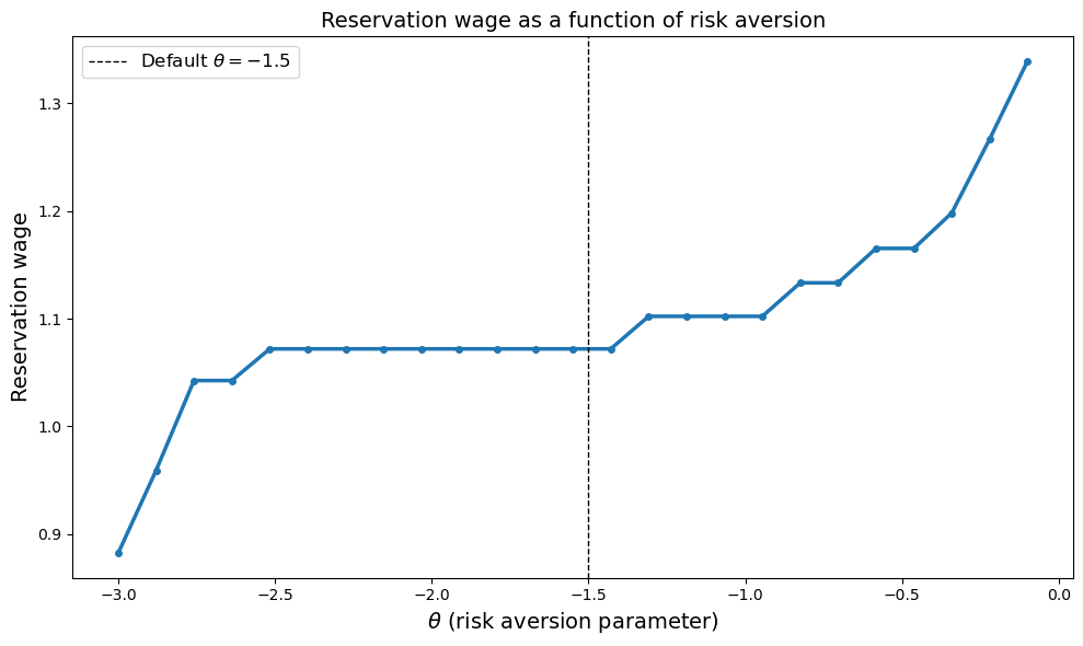
The reservation wage increases as \(\theta\) becomes less negative (moves toward zero)
Equivalently, the reservation wage decreases as the agent becomes more risk averse (more negative \(\theta\)).
The reason is that a more risk-averse agent values the certain income from employment more highly relative to the uncertain future prospects of continued search.
Therefore, they are willing to accept lower wages to escape unemployment.
Exercise 46.2
Use simulation to investigate how the long-run unemployment rate varies with \(\theta\).
Use the parameters from the previous section, where we studied how the reservation wage varies with \(\theta\).
You can use code for simulation from Job Search IV: Fitted Value Function Iteration, suitably modified.
Solution
To compute the long-run unemployment rate, we first write a function to update a single agent.
@jax.jit
def simulate_single_agent(key, model, w_star, num_periods=200):
    """
    Simulate a single agent for num_periods periods.
    Returns final employment status (1 if employed, 0 if unemployed).
    """
    c, α, β, ρ, ν, θ, w_grid, z_draws = model

    # Start from arbitrary initial conditions
    w = 1.0
    status = 1

    def update(t, loop_state):
        w, status, key = loop_state
        key, k1, k2 = jax.random.split(key, 3)

        # Update wage
        z = jax.random.normal(k2)
        w_new = w**ρ * jnp.exp(ν * z)

        # Employment transitions
        sep_draw = jax.random.uniform(k1)
        becomes_unemployed = sep_draw < α

        # Check if unemployed worker accepts wage
        accepts_job = w >= w_star

        # Update employment status
        new_status = jnp.where(
            status,
            1 - becomes_unemployed,   # employed path
            accepts_job               # unemployed path
        )

        new_wage = jnp.where(
            status,
            jnp.where(becomes_unemployed, w_new, w),  # employed path
            jnp.where(accepts_job, w, w_new)          # unemployed path
        )

        return (new_wage, new_status, key)

    init_state = (w, status, key)
    final_state = lax.fori_loop(0, num_periods, update, init_state)
    _, final_status, _ = final_state
    return final_status


def compute_unemployment_rate(model, w_star, num_agents=1000, num_periods=200, seed=12345):
    """
    Compute unemployment rate via cross-sectional simulation.

    Instead of simulating one agent for a long time series, we simulate
    many agents in parallel for a shorter time period. This is much more
    efficient with JAX parallelization.

    The steady state satisfies:
    - Employed workers lose jobs at rate α
    - Unemployed workers find acceptable jobs at rate (1 - F(w*))

    We simulate num_agents agents for num_periods each, then compute
    the fraction unemployed at the end.
    """
    # Create keys for each agent
    key = jax.random.PRNGKey(seed)
    keys = jax.random.split(key, num_agents)

    # Vectorize simulation across agents (parallelization!)
    simulate_agents = jax.vmap(
        lambda k: simulate_single_agent(k, model, w_star, num_periods)
    )

    # Run all agents in parallel
    status_cross_section = simulate_agents(keys)

    # Unemployment rate is 1 - mean(status) since status=1 means employed
    unemployment_rate = 1 - jnp.mean(status_cross_section)

    return unemployment_rate


# Define function to compute unemployment rate for a single theta value
def compute_u_rate_for_theta(θ):
    """Compute unemployment rate for a given theta value"""
    model = create_mccall_model(θ=θ)
    v = vfi(model)
    σ = get_greedy(v, model)
    w_star = get_reservation_wage(σ, model)
    u_rate = compute_unemployment_rate(
        model, w_star, num_agents=5000, num_periods=200
    )
    return u_rate

# Vectorize over theta_grid using vmap
compute_u_rates_vec = jax.vmap(compute_u_rate_for_theta)
unemployment_rates = compute_u_rates_vec(theta_grid)

# Plot the results
fig, ax = plt.subplots(figsize=(10, 6))
ax.plot(theta_grid, unemployment_rates * 100,
        lw=2.5, marker='s', markersize=4)
ax.set_xlabel(r'$\theta$ (risk aversion parameter)', fontsize=14)
ax.set_ylabel('Long-run unemployment rate (%)', fontsize=14)
ax.set_title('Unemployment rate as a function of risk aversion', fontsize=14)
ax.axvline(x=-1.5, color='black', ls='--', linewidth=1, label=r'Default $\theta = -1.5$')
ax.legend(fontsize=12)
plt.tight_layout()
plt.show()
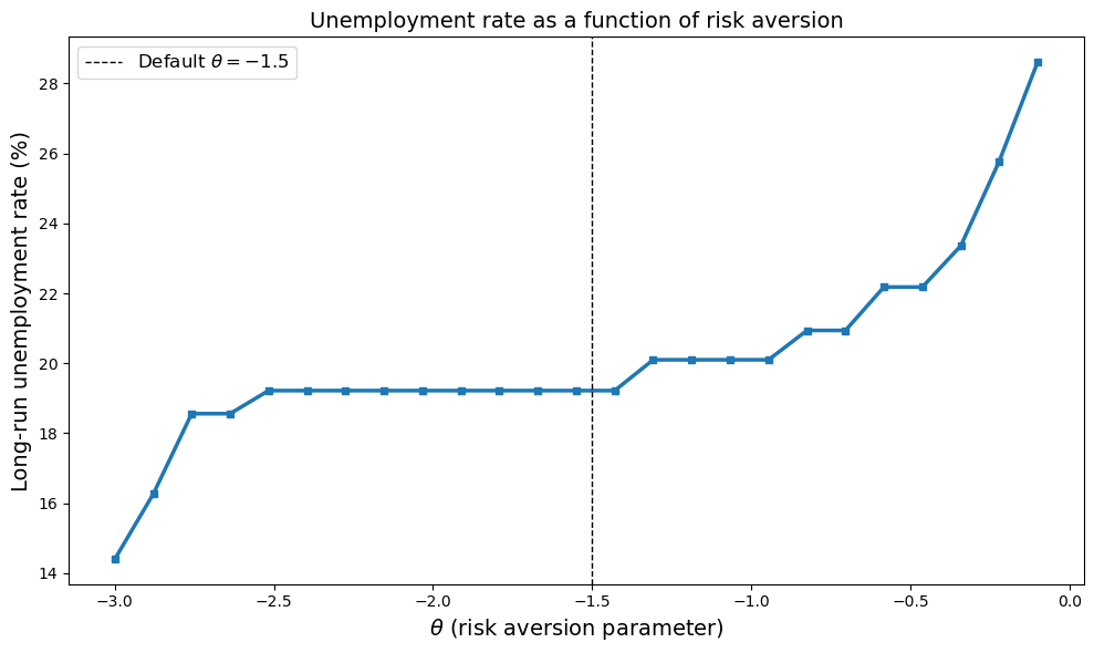
We see that the unemployment rate decreases as the agent becomes more risk averse (more negative \(\theta\)).
This is because more risk-averse workers have lower reservation wages, so they accept a wider range of job offers.
As a result, they spend less time unemployed searching for better opportunities